Measuring Slavery in 2020 Dollars*

by

Samuel H. Williamson
Founder of MeasuringWorth
Miami University
sam@mswth.org

and

Louis P. Cain
Loyola University Chicago
Northwestern University
lcain@northwestern.edu

The initial plan was that indentured servants from the United Kingdom would provide the labor supply in British North America.  After servants completed their indenture contract, they received some land and became free citizens of the colony.  There was also a small number of Africans in 17th century British North America who worked side-by-side with indentured servants.  Little is known about their status before the Virginia slave law of 1661.  Some were treated like servants; others were enslaved.  As the supply of new indentured servants dwindled due to improving conditions in Britain, enslaved Africans became a major source of North American labor in the 18th century. 

In the South slavery became an ingrained economic and legal institution. Slaves and their progeny were the property of an owner, and slaves were owned until they died. They could be bought and sold; their owners controlled their lives and those of their children. When slaves were sold, the contract was a legal document, even to the extent that a buyer could sue the seller if a slave was sold under false pretenses. Even slaves themselves had some protection under the law; they could not be abandoned or executed.

Before independence, the laws of the colonies could not be inconsistent with English law. Chief Justice Lord William Mansfield in the Somersett case (heard in London in 1772) held that English law did not support slavery, a ruling that eventually led to the peaceful extinction of African slavery in the British Empire.¹ By then, the Americans were on a different path. In the Constitutional Convention discussions of 1787, it was held that slavery was not a moral issue but a matter of "interest" only. Some delegates believed that slavery was going to die out. Virginia had attempted several times unilaterally to end the slave trade to Virginia ports, but the Board of Trade lawyers in London had overruled it. The federal government prohibited the trade in slaves beginning in 1808, but statesmanship and jurisprudence could not find a way to end the institution. Within a decade of the Constitutional Convention, Eli Whitney's cotton gin appeared, which is popularly credited with sparking an explosion in cotton production in the South. This explanation may be partly true, but it is also the case that the technological improvements in spinning and weaving in England created a big increase in the demand for cotton, a cloth much preferred to wool. These events together reenergized the demand for slaves.

Slavery is a subject that most Americans have confronted as part of their education, but there are many aspects of slavery that have been left to the dim mists of history. This paper will review some of the basic dimensions of the economics of slavery in the United States and put them in perspective by showing what the financial magnitudes of the "peculiar institution" might be in the relative prices of today. In particular, in 1860 there were nearly four million slaves and their average market value was around $800, but what does that mean?² How much would that be in today's dollars? Answers to such questions are not simple.

Our intention is to present, for the first time, macroeconomic and microeconomic dimensions of slavery in values measured by today's dollars. We are addressing two audiences: the public who know relatively little about these dimensions, and the specialists who may have forgotten that the relative magnitude of these dimensions would be conservatively described as large.

Why does anything have value?

A monetary value can be measured by a transaction when something is bought and sold or as an expected value of an asset currently held. Some assets have value because of the potential income they can generate. An example would be a piece of capital equipment, such as a cotton gin for which planters would pay to have their cotton processed or a slave who would pick the cotton.

Other assets may have value because of their potential resale value, such as land or a rare painting. The owners of a painting choose to have part of wealth invested in something that does not generate current income, either because of an expectation that it will appreciate or because they wish to "consume" the pleasure of owning it. These assets also may give their owner status and power. Owning a Rembrandt painting gives one bragging rights among art collectors. Owning half the acres in the county gives one lots of influence in local politics, regardless of whether the acres are in production or not.

What is the motivation for owning a slave;
what determines the price of a slave at a given point in time?

The demand for a slave is a derived demand, as is that for any productive resource. It is derived from the demand for the output that resource helps to produce. There was an active market for slaves throughout the antebellum period, meaning that slave owners believed the purchase of a slave would prove to be a profitable expenditure, even though that expenditure required a considerable amount of money.³  As we will explain below, at the time the South seceded from the Union, the purchase of a single slave represented as much as $180,000 and more in today's prices. This was twice the average of 14 years earlier, indicating a sustained growth in the demand for slaves. Economists would say that these observations alone indicate that the profitability of "investing" in a slave was increasing substantially.

Why would a slave have so much value? A short answer is the value of a slave is the value of the expected output or services the slave can generate minus the costs of maintaining that person (i.e., food, clothing, shelter, etc.) over his or her lifetime.⁴ A quick list of the data that have to be considered in determining the value of a slave's expected revenue would include sex, age, location, how much he or she is likely to produce (a factor that included a slave's health and physical condition), and the price of the output in the market. For a female slave, an additional thing to consider would be the value of the children she might bear.

In addition, there is considerable evidence that slaves were worked harder than free labor in Southern agriculture; what slaves could be induced to produce in bondage was greater than what they could be expected to produce with the freedom to make their own choice of labor or leisure.⁵

As these outputs and costs are in the future, they must be discounted to their present value, so an owner must choose a discount rate. And, as they are in the future, there is uncertainty in determining what they are, so the present value of a slave is an estimate made by the current or a prospective owner.⁶ In general, most economic historians believe that slavery was profitable, even at these expensive prices.

Figure 1 demonstrates how the price of slaves varied with respect to age, sex, and location during the antebellum period. As one can see, prices were higher in the New South than in the Old South (the states along the Atlantic coast) and higher for males than for females.⁷ The statistics on slave prices show that healthy young adult men in the prime of their working lives had the highest price, followed by females in the childbearing years. Young adult males had more value as they were stronger, could work harder in the fields, and could be expected to work at such a level for more years. Young adult women had value over and above their ability to work in the fields; they were able to have children who by law were also slaves of the owner of the mother. Old and infirm slaves had low, even "negative," prices because their maintenance costs were potentially higher than the value of their production. Similarly, young children had low prices because the "cost" of raising them usually exceeded their annual production until they became teenagers.

Figure 1

Age-Sex Profile of Slave Values
Louisiana Male 18-30 = 100

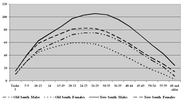
Source: Source: Historical Statistics, Table Bb215-218. Index of slave values, by age, sex, and region: 1850. All the values are indexed to that of Louisiana males aged 18-30.

Those who have researched slave prices have discovered that a large number of additional variables went into the determination of the price of any particular slave at a particular point in time. A premium was paid if the slave was an artisan -- particularly a blacksmith (+55%), a carpenter (+45%), a cook (+20%), or possessed other domestic skills (+15%). On the other hand, a slave's price was discounted if the person was known to be a runaway (-60%), was crippled (-60%), had a vice such as drinking (-50%), or was physically impaired (-30%). In general, the discount for each of the slaves was slightly larger for females than for males.⁸ The prices presented above are average prices for the slaves transacted in a given year. A person studying their family's history might come across a notation that a family member purchased a slave at a given price or that a former slave purchased his or a family member's freedom at a given price. Without information regarding these details, it is difficult to interpret what the price of a single slave means.

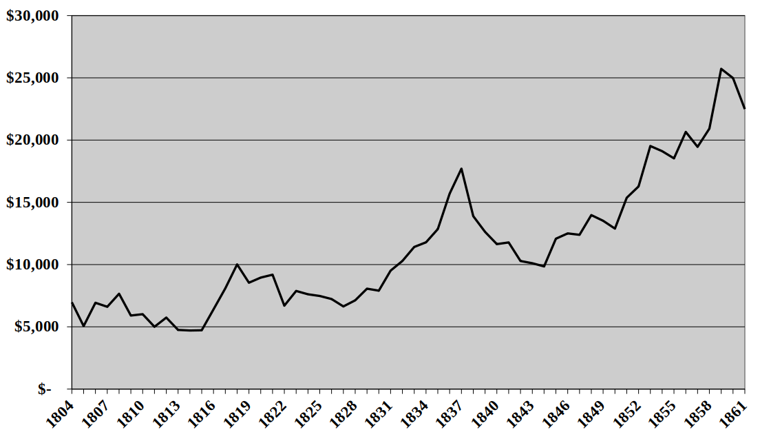
The path of the average of slave prices can be seen in Figure 2. While much of the movement can be explained by what is happening in the cotton market, the first two spikes are also related to general economic conditions. During and after the War of 1812 there was a 40% increase in all prices, with the price of raw cotton more than doubling during the same period. In the 1830s, the price of slaves increased quickly due to expectations bred by discussions to refund the federal budget surplus to the states. Discussions about "internal improvements" (e.g., canals and railroads) led to a boom in land prices and, once again, cotton prices. After the "Panic of 1837" there was a long depression. Finally, the almost three-fold increase in prices after 1843 can be explained by several factors, including the rapid increase in the worldwide demand for cotton and increased productivity in the New South attributable to better soil and improvements in the cotton plant. It is clear during this time that the market for slaves was active, and that slaves were regarded as more valuable.

Figure 2

Average Price of a Slave Over Time
Current dollars

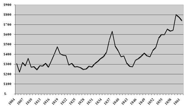
Source: Historical Statistics, Table Bb212. Average Slave Price.

What is the comparable "value" of a slave in today's prices?

None of these prices has much meaning to us today, but they would if we revalue them in today's dollars to the amount of money slave owners spent 170 years ago.⁹ The techniques developed in MeasuringWorth have created four "measures" to use to compare a monetary value in one period to one in another, as explained in the essay "Measures of Worth."¹⁰ Of these ten, three are useful for discussing the value of a slave. They are: labor or income value, relative earnings and real price.¹¹ Using these measures, the value in 2020 of $400 in 1850 (the average price of a slave that year) ranges from $14,000 to $240,000. We use the 1850 price in our example, as that was close to the average price for the entire antebellum period.

Labor or Income Value

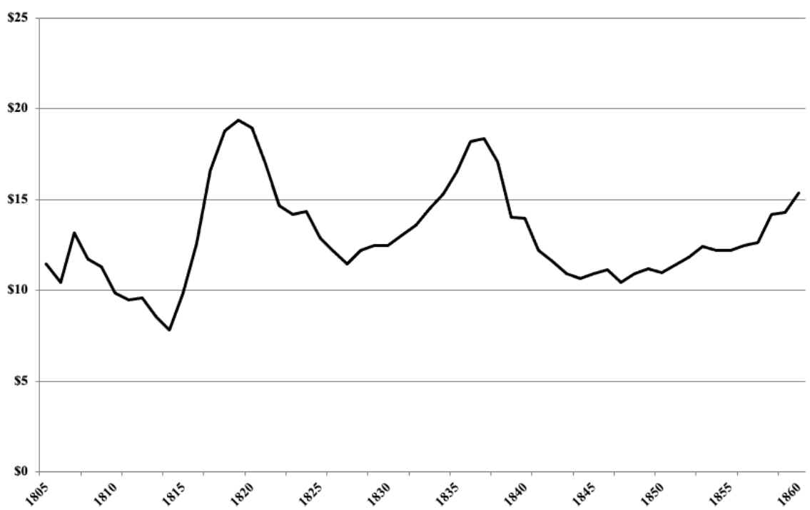
As discussed above, the $400 price in 1850 represents the expected net value of the future labor services a slave would provide. Most slaves worked on the farms and plantations of their owners, although some slaves were rented out for farm and other types of work. In either case, the work they did was mostly unskilled. So, a comparable measure of the value of these services is reflected in the unskilled wage.¹² That is why the labor or income value, using the unskilled wage is the best measure of the value of a slave's services in today's prices. That $400 would be $114,000 in today's price.  As Figure 3 shows during the antebellum period, the value in in today's dollars. of a slave ranged from $60,000 (in 1809) to $184,000 (in 1859).

Figure 3

Labor Income Value
of Owning a Slave in 2020 Prices

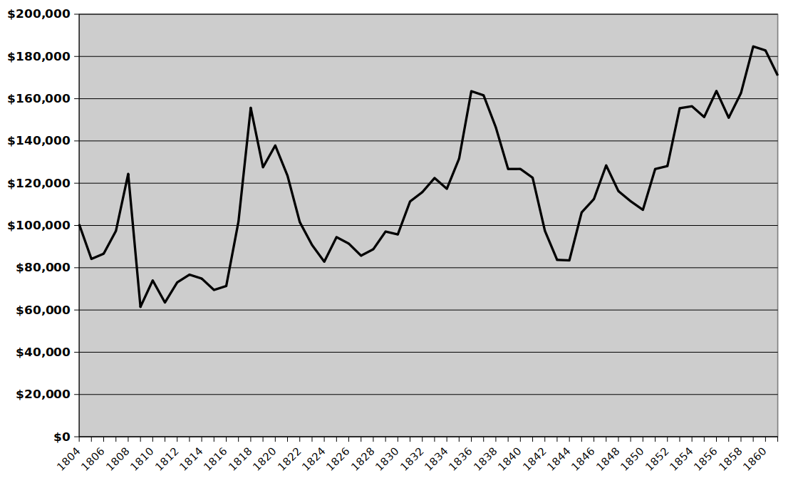
In other words, we can assume that the unskilled wage a free employee would have received to do similar work to that of a slave is a reasonable approximation of the value slaveowners imputed for labor in the price of a slave. To be clear, this calculation is not the present value of what one would have to pay a free laborer to do the work of a slave then or now. Recall that the price of a slave measures the average present value of the net return over that slave’s life expectancy. Slaves received room, board and clothing, but they were responsible for producing a large portion of those items. Slaves were driven to produce a greater output than they would have produced had they been free. Finally, the work week has become shorter and life expectancy longer than in the mid-1850s. This calculation uses the unskilled wage to give an approximation of what it cost to acquire a slave then in today’s dollars.

Remarkably, even at these prices, some slaves, mainly those with artisan skills, might ultimately earn enough to buy themselves and perhaps their family out of slavery. It was not uncommon, especially in the Old South, for masters to allow others to hire the services of his or her slaves. This was particularly true of slaves who lived in urban areas, independent of the master. They were expected to make their own arrangements. "The master fixed the wage that the slave must bring in. All above this amount the slave might keep himself. Employers frequently hired the slave's time from the owner at a certain amount and paid the slave an additional wage contingent on the amount of work accomplished."¹³

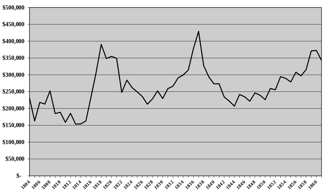
Relative Earnings

The $400 average slave price in 1850 can also be thought of as a signaling device of status in a period where the annual per capita income was about $110. Relative earnings can be viewed as the ability to purchase expensive goods. Today, the middle and upper-middle classes aspire to goods and services such as a second home, and an expensive car as a way of showing others that they have "arrived"-- that they have achieved some status in the economy. The average slave price in 1850 was roughly equal to the average price of a house, so the purchase of even one slave would have given the purchaser some status. The calculation of relative earnings is based on the ratio of GDPs per capita.¹⁴ Consequently $400 in those days corresponds to nearly $240,000 in relative earnings today (see Figure 4.) While it might be better to make the comparisons using average wealth then and now, those numbers are not available. There is evidence, however, that wealth and income are closely related and move up and down together.

Figure 4

Relative Earnings
of Owning a Slave in 2020 Prices

Real Price

Economists commonly use the real price measure when they are trying to account for the impact of inflation. The real price today is computed by multiplying the value in the past by the increase in the consumer price index (CPI). The result compares that past value to a ratio of the cost of a fixed bundle of goods and services the average consumer buys in each of the two years. In the construction of the CPI bundle, an effort is made to compensate for quality changes in the mix of the bundle over time.¹⁵ Still, the longer the time span, the less consistent the comparison. In the 19th century, there were no national surveys to figure out what the average consumer bought, and slaves were not a consumption good. The earliest budget study used by economic historians was of 397 workmen's families in Massachusetts and was constructed in 1875. These families spent over half their income on food and rented their housing.¹⁶

The MeasuringWorth calculator shows that the "real price" of $400 in 1850 would be approximately $13,500 in 2020 prices (see Figure 5). We all can identify with what that amount of money would buy today, but hardly anything we would spend $13,500 on today was available 170 years ago. $400 in 1860 would have purchased 4,800 pounds of bacon, 3,000 pounds of coffee, 1,600 pounds of butter, or 1,000 gallons of gin. It is unlikely, however, that this was the budget of the typical slave owner. Most of the food would be produced on the plantation, and housing would have been buildings constructed by the owner (and his slaves). The "opportunity cost" of the $400 for the slave owner would have been supplies for the plantation, or perhaps luxuries and travel.

Figure 5

The Real Price of Owning a Slave
in 2020 Dollars

Using the real price is not the correct index to use for measuring the value of a slave's labor services in today's prices. It does, however, give an idea of what the cost of purchasing a slave was in 2020 dollars. Thus, just before the start of the Civil War, the average real price of a slave in the United States was $25,000 in current dollars. There is ample evidence that there are several million of people enslaved today, even though slavery is not legal anywhere in the world. There are several organizations such as Anti-Slavery International that will point out that in many places today, slaves sell for as little as (or even less than) $100!

What was the distribution of slave ownership?

A second issue of interest is slave wealth in both micro- and macro-economic terms. Slaveholders were wealthy individuals both with respect to other Southerners and with respect to the whole country. At the time, the Census Bureau measured wealth in two forms: real estate and personal estate. The land and buildings of a slave plantation were real estate; the slaveholdings were part of personal estate. Together they sum to Total Estate.   On both dimensions, slaveholders were different from other Southerners. The average white Southern family in antebellum America lived on a small farm without slaves. Slave ownership was the exception, not the rule.

Let us begin by looking at land. Lee Soltow collected the data by "spin" sampling from the 1860 census.¹⁷ Following the US census, he defined a farm as involving at least 3 improved acres of land, and it should be noted that this is for farms throughout the United States, not just the South. The size distribution of farms is shown in Table 1.

"Number" is the number of farms in the interval. The stereotypical picture of slavery is that it involved a large plantation. Farms that were greater than 500 acres (there are 640 acres in a square mile) comprise just 1.31 percent of farms. The vast majority of farms were between 20 and 500 acres.

Table 1

Size Distribution of Farms - 1860 for farms of 3 or more improved acres)
acres	number	percent	cum %	cum %
>1000	5,364	0.27	100.00	0.27
500 - 999	20,319	1.04	99.73	1.31
100- 499	487,041	24.91	98.69	26.23
50 - 99	608,878	31.14	73.77	57.37
20 - 49	616,558	31.54	42.63	88.91
10 - 19	162,178	8.30	11.09	97.20
3 - 9	54,676	2.80	2.80	100.00
Source: Soltow, table 5.1

Table 2 shows that the distribution of slave ownership in Soltow's data is more skewed than land.

Table 2

Disbribution of Slaves and Estate Value among Free Adult Males in South - 1860
Number of	Number			Total
slaves	slaveholders	percent	cum %	Estate
>1000	1	0.00005	100.00
500 - 999	13	0.00065	100.00	$957,000
100 - 499	2,278	0.11	100.00	$160,000
50 - 99	8,367	0.42	99.88	72,000
10 - 49	97,333	4.89	99.46	17,200
5 - 10	89,556	4.50	94.57	$8,800
1 - 4	187,336	9.41	90.07	$3,670
0	1,605,116	80.66	80.66	$-
Source: Soltow (1975), table 5.3

By 1860, over 80 percent of the free adult males in the South did not own slaves. Only 0.11 percent owned more than 100. The Total Estate for those in the upper tail of the distribution was enormous. It should be emphasized that this is not a small elite; as a group, slave owners were sizeable and wealthy. Those with more than 500 slaves were essentially millionaires in the current dollars of 1860. Some of these slaveowners were women.¹⁸

Soltow calculated the Total Estate for free adult males at each of the break points in the distribution of slaves reported above. Soltow reports that the average Total Estate in the South in 1860 was $3,978, as compared to just $2,040 in the North.¹⁹ Given that the average slave price in 1860 was $800, if Southern wealth was exclusively slaves, that amount would equate to just over 5 slaves. Total Estate, however, also includes real estate, and Soltow reports that amount actually involves an average of 2 slaves. Thus, according to the table above, 90.07 percent of free adult males in the South owned fewer slaves than implied by average wealth. In 1860, the top one percent of wealth holders held 27 percent of Total Estates; the bottom 50 percent held but one percent of the total.

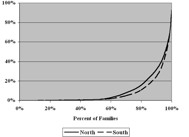
In Figure 6 below, we see how the distribution of Total Estate in the South compared to that in the North in 1860. The data again come from Soltow's sampling. As one can see, there is almost no difference between the North and the South at the top of the distribution. The North is slightly above the South at the 0.001 level, but they are even at the 0.01 level. The largest planters were as wealthy as the major Northern merchants and industrialists. Between .01 and .10 levels, the South forges ahead before the North begins to close the gap. In both areas, the bottom 50% of the wealth distribution held but 1% of measured wealth. The evidence suggests that a Southern white farm family of four (a husband, wife, and two children) who owned a slave family of four had more wealth than a Northern white farm family of four that employed a couple of farm laborers. Non-slaveowners in the South were probably little different from Northern farmers. The aggregate share of the top 10% of the wealth distribution of Southern wealth is seven percentage points more than the top 10% of the Northern distribution (75% vs. 68%).

Figure 6

Wealth Distribution 1860
North vs. South

What is the comparable "value" of the wealth in slaves in today's prices?

Of the ten "measures" developed by MeasuringWorth, two are useful for discussing the value of the wealth invested in slaves. They are relative earnings and relative output. We discussed the concept of relative earnings in relation to evaluating a slave's price above, but it is also useful for discussing wealth, as people with high relative earnings are typically people of wealth.

Relative Output

The people who are the financial and political leaders of a community are often its most wealthy. Even if they have not been elected to power, the wealthy often have disproportionate influence on those who do. Relative output measures the amount of income or wealth compared to the total output of the economy. Those individuals with considerable income or wealth are more likely to be able to influence the composition or total-amount of production in the economy.

The relative output of a $400 slave in 1850 would be $3.4 million today. While this number seems very large, as we will show below, the wealth tied up in slaves was a large proportion of the total wealth of the nation. Slave owners as a group had considerable economic power. It  is interesting to note that the relative output of owning one slave was as high as $14 million in 1818. This finding is consistent with the history of the period when southern states exercised great influence on such issues as tariffs, banking, and in which new areas of the country slavery would be allowed.  As the century progressed, the political influence possessed by slave owners  declined because industrialization and agriculture in the North grew faster than the slave economy.

The Total Estates of slave owners were quite large, as is demonstrated when measured in current dollars. Table 3 shows the relative earnings and relative output of their estates in 2020 dollars.

Table 3

Distribution of Total Estate among Slaveholders
Number of Slaves	Total Estate (thousands of 1860 Dollars)	Relative Earnings  (millions of 2020 $)	Relative Output  (millions of 2020 $)
>1000	NR	-	-
500 - 999	$         957	$        458	$     4,810
100 - 499	$         160	$          77	$        804
50 - 999	$           72	$         34	$        361
10 - 49	$           17	$            8	$          85
5 - 10	$             9	$            4	$          45

Comparing these two tables, it becomes quite clear that the holder of 10 slaves likely ranks in the top one percent of the distribution, if relative earnings is used as the standard of comparison. Potentially all slaveholders rank in the top one percent, if relative output is used as the standard of comparison. Clearly, the ownership of even one slave implied that the owner was a wealthy member of the community. Those who owned over 500 slaves had a measure of relative output that compares to billionaires today.

How much wealth was invested in slaves?

Slaves had an important impact on the differences in regional wealth. Gavin Wright made estimates of both Northern and Southern wealth. His data for 1850 and 1860 are reported in  Table 4 below. The "value of slaves" figures are taken from Sutch and Ransom (1988).²⁰

Table 4

	Regional Wealth in 1850 and 1860 Millions of dollars (except per capita)
	North	South	North	South
	1850	1850	1860	1860
Total Wealth	$4,474	$2,844	$9,786	$6,332
Value of Slaves		$1,286		$3,059
Non-slave Wealth	$4,474	$1,559	$9,786	$3,273
Wealth (free) per capita	$315	$483	$482	$868
Non-slave (free) Wealth per capita	$315	$174	$482	$294
Source Wright (2006), p. 60.

A significant proportion of the wealth of slave owners was eliminated by the stroke of Abraham Lincoln's pen when he signed the Emancipation Proclamation that freed slaves in the rebellious areas. Success on the battlefield ensured their freedom. Remember that the Emancipation Proclamation freed slaves only in areas in rebellion not all slaves. More fundamentally, it was success on the battlefield that eliminated this wealth. Total slave wealth was immense. Figure 7 shows the aggregate value of slaves adjusted to today's prices measured using the relative share of GDP. While it varies with the price of slaves over the period, it is never less than six trillion 2020 dollars and, at the time of Emancipation, was close to thirteen trillion 2020 dollars.

Figure 7

Wealth in Slaves in Trillions of 2020 dollars
As Measured by the Share of the GDP

An alternative way of making that calculation is to use Soltow's finding that Total Estate in slaves was 15.9 percent of the 1860 total.²¹ The Federal Reserve's Flow of Funds accounts report net worth for households is about $121 trillion in 2020. If Soltow's percentage is applied to that data, the result is again approximately $14 trillion. In case anyone think that a relatively small number, it is roughly 77 percent of GDP today.

If Wright's figures above are adjusted to today's prices through the use of the relative share of GDP measure, they tell the same story as the Table 5 below shows.

Table 5

	Regional Wealth in 1850 and 1860 Billions of $2020 dollars
	North	South	North	South
	1850	1850	1860	1860
Total Wealth	$37,300	$23,700	$48,000	$31,000
Value of Slaves	-	$10,700	-	$15,000
Non-slave Wealth	$37,300	$13,000	$48,000	$16,000

It should be noted that wealth grows roughly 30 percent over the decade of the 1850s in both the North and South. However, in the South, the value of slaves grew about 40 percent over the decade, while non-slave wealth grew at only about 25 percent.²² Some economic historians have hypothesized that Southerners had so much wealth tied up in slaves that they did not invest sufficiently in other types of investments. This is a concept called "crowding out." Whether that is the reason or not, it is clear at the start of Civil War, the North had three times the amount of non-slave wealth as the South, and this discrepancy would be at least partly represented in factories and other capital that was an advantage in waging a war.

Conclusions

Slavery in the United States was an institution that had a large impact on the economic, political and social fabric on the country. This paper gives an idea of its economic magnitude in today's values. As noted in the introduction, they can be conservatively described as large.

Bibliography

Carter, Susan B., Scott Sigmund Gartner, Michael R. Haines, Alan L. Olmstead, Richard Sutch and Gavin Wright, editors, Historical Statistics of the United States: earliest times to the present (New York: Cambridge University Press, 2006).

Conrad, Alfred, and John Meyer. "The Economics of Slavery in the Antebellum South." Journal of Political Economy, vol. 66, no. 2, April 1958.

David, Paul, Herbert Gutman, Richard Sutch, Peter Temin, and Gavin Wright. Reckoning with Slavery: A Critical Study in the Quantitative History of American Slavery. New York: Oxford University Press, 1976.

Fogel, Robert William. "A Comparison between the Value of Slave Capital in the Share of Total British Wealth (c.1811) and in the Share of Total Southern Wealth (c.1860)," chapter 56 of Robert William Fogel, Ralph A. Galantine, and Richard L. Manning, Without Consent or Contract: Evidence and Methods. New York: Norton, 1992.

Fogel, Robert William. Without Consent or Contract: The Rise and Fall of American Slavery. New York: W. W. Norton, 1989.

Fogel, Robert William, and Stanley Engerman. Time on the Cross: The Economics of American Negro Slavery, 2 vols. Boston: Little, Brown, 1974.

Gray, Lewis Cecil, History of Agriculture in the Southern United States to 1860. Baltimore: Waverly Press, 1933, p. 566

Kotlikoff, Laurence J. "Quantitative Description of the New Orleans Slave Market, 1804 to 1862," chapter 3 of Robert William Fogel and Stanley L. Engerman, Without Consent or Contract: Markets and Production: Technical Papers, Volume 1 (New York: Norton, 1992), reprinted from Economic Inquiry, vol. 17, no. 4, October 1979.

Jones-Rogers, Stephanie, They Were Her Property: White Women as Slave Owners in the American South. New Haven, Yale University Press, 2019

Officer, Lawrence H. and Samuel H. Williamson "What Was the Value of the US Consumer Bundle Then?" MeasuringWorth, 2021. URL: http://www.measuringworth.org/consumer/

Officer, Lawrence H. and Samuel H. Williamson "The Annual Consumer Price Index for the United States, 1774-Present," MeasuringWorth, 2020 URL: http://www.measuringworth.org/uscpi/

Olmstead, Alan, and Paul Rhode, Creating Abundance: Biological Innovation and American Agricultural Development. New York, Cambridge University Press, 2008.

Ransom, Roger and Richard Sutch, "Capitalists without Capital: The Burden of Slavery and the Impact of Emancipation," Agricultural History 62 (3) (1988)

Soltow, Lee, Men and Wealth in the United States 1850-1870 (New Haven: Yale University Press, 1975).

Williamson, Samuel H. and Louis Cain " Defining Mesures of Worth," MeasuringWorth, 2023. URL http://www.measuringworth.com/defining_measures_of_worth.php

Wright, Gavin. Slavery and American Economic Development. Baton Rouge: Louisiana State University Press, 2006.

 

---

* The authors thank Stanley Engerman, Richard Sutch, Robert Whaples and Gavin Wright for their comments on a previous drafts. The Previous versions:
Measuring Slavery in 2009 Dollars
Measuring Slavery in 2016 Dollars
Back to text

¹
See The Somerset vs Stewart Case.
Back to text

² Susan B. Carter, Scott Sigmund Gartner, Michael R. Haines, Alan L. Olmstead, Richard Sutch and Gavin Wright, editors, Historical Statistics of the United States: earliest times to the present (New York: Cambridge University Press, 2006), series Bb212.
Back to text

³ Between 1804 and 1862, 135,000 slaves were sold on the New Orleans market. Kotlikoff, "Quantitative Description of the New Orleans Slave Market, 1804 to 1862" (1979)
Back to text

⁴ These costs are an obligation of the slave owner even when the slave is too young, old or infirm to work. There is ample evidence that these slaves who were not productive did not receive as much food as the able bodied, but there is no evidence that they were allowed to starve.
Back to text

⁵ See Robert William Fogel, Without Consent or Contract: The Rise and Fall of American Slavery (New York: W. W. Norton, 1989), Chapter 3.
Back to text

⁶ Present value is the value today of a series of payments, or a single payment, that will be received in the future. Money put in a bank or alternative investment today will grow over time depending on the interest rate. What is received in the future is principle plus interest. Present value calculations determine the amount of principle that is needed today in order to realize a given series of payments in the future.
Back to text

⁷ The main reason that New South Slaves had higher prices was that the soil was more fertile there, so plantations were more productive. See Alan Olmstead and Paul Rhode, Creating Abundance: Biological Innovation and American Agricultural Development (New York: Cambridge University Press, 2008).
Back to text

⁸ See Fogel, op. cit., pp. 69-70.
Back to text

⁹ Of course, the number had different meaning to the slave. However, as there were cases where slaves bought their own freedom, the opportunity cost question is the same.
Back to text

¹⁰Samuel H. Williamson, and Louis P. Cain. Defining Mesures of Worth," MeasuringWorth, 2023. URL: https://www.measuringworth.com/defining_measures_of_worth.php
Back to text

¹¹ A fourth measure, relative output, is used in our discussion of the magnitude of the wealth represented by the ownership of slaves.
Back to text

¹² In his famous history of Agriculture in the Southern United States to 1860 (Washington, D.C.: Carnegie Institution, 1933), Gray writes "Planters preferred to employ their own slaves rather than hire them to others. Because of the scarcity of efficient white labor, demand for Negro artisans was usually considerable, and good wages were offered for their services. Unskilled labor was in demand for lumbering, mining, the constructions of canals and railways, steamboating, dock labor, and other 'public works.'" p. 566
Back to text

¹³ Lewis Gray, op. cit, p. 566
Back to text

¹⁴ Given that GDP for 2020 reflects the short-lived, pandemic-caused recession, for the calculations in this paper we use the 1st quarter estimate of GDP for 2021 as better reflecting the long-term trend. Nominal GDP fell roughly 2.3% in 2020; the 1st quarter estimate for 2021 is 2.9% greater than that for 2019.
Back to text

¹⁵ See Lawrence Officer, "What Was the Value of the US Consumer Bundle Then?" MeasuringWorth, 2009a,and Offficer, "The Annual Consumer Price Index for the United States, 1774-Present," MeasuringWorth, 2009b.
Back to text

¹⁶ Today the share of food and beverages of the average household is 15% and most of the cost of housing is to maintain a residence that is owned.
Back to text

¹⁷ Lee Soltow, Men and Wealth in the United States 1850-1870 (New Haven: Yale University Press, 1975).
Back to text

¹⁸ See Jones-Rogers, Stephanie, They Were Her Property: White Women as Slave Owners in the American South (New Haven, Yale University Press, 2019)
Back to text

¹⁹ Soltow, op. cit., p. 181.
Back to text

²⁰ That amount of wealth in slaves was calculated by Roger Ransom and Richard Sutch as the product of a three-year moving average of slave prices and the size of the slave population.
Back to text

²¹ Most economic historians feel the slave prices in 1860 were artificially high for a variety of reasons and that even without the War, they would have fallen, so these comparisons of wealth somewhat overstate the wealth of the South at the time.
Back to text

²² The percent figure was calculated by Fogel from Soltow: Robert W. Fogel, "A Comparison between the Value of Slave Capital in the Share of Total British Wealth (c.1811) and in the Share of Total Southern Wealth (c.1860)," chapter 56 of Robert William Fogel, Ralph A. Galantine, and Richard L. Manning, Without Consent or Contract: Evidence and Methods (New York: Norton, 1992.
Back to text

---

Please let us know if and how this discussion has assisted you in using our calculators.